Chapter: Statistics - Class 10

Statistics is the study of collecting, analyzing, interpreting, presenting and organizing data. It involves methods to gather information from datasets, summarize findings using measures like averages or percentages and draw conclusions or make predictions based on that information. This chapter includes various methods of measuring central tendency such as arithmetic mean, median, mode, empirical formula, bar graphs, histogram, pie chart, frequency polygon and ogive.

Data

Frequency

Grouped Data and Class Interval

Class Mark

Arithmetic Mean or Mean

Median

Mode

Empirical Formula

Quartiles

Graphical Representation

Solved Questions Based on Statistics

Data

Data refers to information or facts that are collected, observed or recorded. It can be in the form of numbers, words, measurements, or observations about people, events, things, or phenomena.

Raw Data

Raw data refers to the original, unprocessed information collected directly from observations, measurements, or recordings.

Frequency

Frequency refers to the count or number of times a particular value, category, or event occurs in a dataset. The frequency of data is represented by f.

For example The alphabet ‘s’ appears three times in the word statistics, thus the frequency of ‘s’ is 3.

Cumulative Frequency

Cumulative frequency refers to the total of frequencies or counts of values within a dataset. It represents the sum of frequencies up to a certain point in a data distribution. As each value is added, the cumulative frequency continuously increases.

For example: The shoe sizes of ten students of Class IX are 6, 8, 9, 7, 6, 7, 9, 6, 10, 8.

Cumulative frequency distribution table:

Shoe Size	Frequency	Cumulative Frequency
6	3	3
7	2	3+2=5
8	2	5+2=7
9	2	7+2=9
10	1	9+1=10

Notice that the final cumulative total will consistently match the total for all observations because each frequency has already been included in the preceding total.

Grouped Data and Class Interval

Grouped data refers to a method of organising a large set of numerical data into intervals or ranges, rather than listing individual values. This grouping allows for easier analysis and presentation of data when dealing with a wide range of values.

Class intervals are the ranges or divisions into which the data is grouped. They are created by grouping data values into categories or intervals of equal width or size.

Lower Limit and Upper Limit

The lower limit is the smallest value or the starting point of a class interval. It defines the lowest value included in a particular interval.

The upper limit is the largest value or the endpoint of a class interval. It defines the highest value included in that interval.

For Example, in a grouped frequency distribution where data is grouped into intervals if an interval is defined as 25- 35, the lower limit is 25 and the upper limit is 35.

Class Mark

The class mark of a class interval is the middle value within that interval. It is calculated as the average of the lower and upper limits of the interval.

Class Mark = (Lower limit + Upper limit) / 2

For example, What will be the class mark of the given class: 10 − 20?

Lower limit = 10
Upper limit = 20
Class mark = (Lower limit + Upper limit) / 2
                 = (10 + 20) / 2
                 = 30 / 2
                 = 15

Measures of Central Tendency

Measures of central tendency are numerical expressions that represent the characteristics of a dataset. There are many types of statistical averages such as arithmetic mean or mean, median and mode.

Arithmetic Mean or Mean

The arithmetic mean is the arithmetic average of all the values in a dataset. It's calculated by adding up all the values and dividing by the number of values. 

The mean of n observations is

Mean = (Sum of all observations) / (Total no. of observations)

Example: The weight (in kgs) of 5 students is 45.5, 52, 55, 65 and 49.5. What is the arithmetic mean of their weight?

a) 53.8 kg
b) 53.6 kg
c) 53.2 kg
d) 53.4 kg

Answer: d) 53.4 kg

Explanation: The arithmetic mean is the arithmetic average of all the values in a dataset. 

Mean = (Sum of all observations) / (Total number of observations)
         = (45.5 + 52 + 55 + 65 + 49.5) / 5
         = 267 / 5
         = 53.4 kg

Arithmetic Mean of Tabulated Data

The arithmetic mean for a given discrete frequency distribution can be obtained by using one of the three methods:

(i) Direct method

The formula for finding the mean by the direct method is

Where

x is the variate.

f is the frequency.

Σf_ix_i is the sum of the product of each x and its frequency f.

Σf_i is the total of all frequencies.

i varies from 1 to n

(ii) Assumed Mean method

The formula for finding the mean by the assumed mean method is

Where

x is the variate.

f is the frequency.

A is the assumed mean.

deviation (d_i) = x_i − A

Σf_id_i is the sum of the product of each deviation d and its frequency f.

Σf_i is the total of all frequencies.

i varies from 1 to n

Example: The weight of 40 students of a class is given below:

Weight (in kg)	55	57	59	61	63
No. of students	8	11	9	7	5

What is the mean weight of the students using the assumed mean method?

a) 58.5 kg
b) 58.25 kg
c) 58.75 kg
d) 58 kg

Answer: a) 58.5 kg

Explanation: Steps for finding the mean using the assumed mean method are:

a. Create a four-column frequency table.

(i) Enter the variate (x_i) values in the first column from the left.

(ii) Record the frequency (f_i) of each variate in column (a) in the second column from the left.

b. Select a number, 'A' (ideally from the variate ‘x_i’ values that are provided in the first column). In this case, 'A' is referred to as the assumed mean.

To obtain the deviation 'di,' subtract the assumed mean 'A' from each value of variate 'x_i' in the first column.

Thus, deviation (d_i) = xi − A

In the third column, record the values of each deviation (d = x − A) together with the matching frequencies.

c. To obtain the values of fidi, multiply the frequency (f_i) in the second column by the matching deviation (d_i) in the third column.

Record the values of fidi in the fourth column and against the corresponding values of deviations 'di'.

d. Determine ∑f_id_i, the total of all the values of f_id_i in the fourth column.

Also, ∑f_i = n, the sum of all values of frequency ‘f_i’.

e. The following formula gives the required mean using the assumed mean method:

Let assumed mean (A) = 59

Thus,

Weight (in kgs) (xi)	No. of Students (fi)	di = xi − A = xi − 59	fidi
55	8	− 4	− 32
57	11	− 2	− 22
59	9	0	0
61	7	2	14
63	5	4	20
Σfi = 40	Σfidi = − 20

Mean = A + ^Σf_id_i⁄_Σfi
         = 59 + ^(-20)⁄₄₀
         = 59 - 0.5
         = 58.5 kg

(iii) Step-deviation method

The following formula gives the required mean using the step-deviation method:

Where

x is the variate.

f is the frequency.

A is the assumed mean.

t_i = (x_i − A) / h

Σf_it_i is the sum of the product of each t and its frequency f.

Σf_i is the total of all frequencies.

h is the biggest integer that divides (x_i − A)

i varies from 1 to n.

Mean of Grouped Data (both continuous and discontinuous)

(i) Direct Method

Steps:

1. Find the mid-value of each class interval.
2. Represent the mean value by x.

The formula for finding the mean by the direct method is

Mean = ^Σf_ix_i⁄_Σfi

Where

x is the variate.

f is the frequency.

Σf_ix_i is the sum of the product of each x and its frequency f.

Σfi is the total of all frequencies.

i varies from 1 to n.

(ii) Assumed Mean Method

Steps:

1. Find the mid-value of each class interval.
2. Represent the mean value by x.

The formula for finding the mean by the assumed mean method is

Mean = A + ^Σf_idi⁄_Σfi

Where

x is the variate.

f is the frequency.

A is the assumed mean.

deviation (d_i) = A − xi

Σf_id_i is the sum of the product of each deviation d and its frequency f.

Σf_i is the total of all frequencies.

Note:

Any number can be taken as the assumed mean but to make the calculations easier, it should be taken from the middle of the values of x.

(iii) Step-deviation method

According to this method,

Mean = A + (^Σf_it_i⁄_Σfi × h)

Where

A is the assumed mean.

ti = (x_i − A) / h

h = class size

i varies from 1 to n

Median

When data is arranged in an order, the middle value is known as the median. The data can be arranged in ascending or descending order. 

Median for Raw Data

Let there be n terms and they are arranged in ascending or descending order.

(i) If n is odd, then median = (ⁿ⁺¹⁄₂)^th term

(ii) If n is even, there are two middle terms, that is (ⁿ⁄₂)^th term and (ⁿ⁄₂ + 1)^th term.

Thus, the median is the arithmetic mean of these two terms.

Example: What is the median of 11, 7, 14, 22, 9, 5 and 12?

a) 5
b) 12
c) 11
d) 9

Answer: c) 11

Explanation: We know that the median is the middle value in a dataset when arranged in ascending or descending order.

Thus, arranging the given terms in ascending order according to their magnitudes.

5, 7, 9, 11, 12, 14, 22

Since there are an odd number of values, then median = (ⁿ⁺¹⁄₂)^th term

Where

n is the total number of terms.

n = 7

Thus, median =  (⁷⁺¹⁄₂)^th term
                     = (8 / 2)^th term
                     = 4^th term

Thus, median = 11

Median for Tabulated data

Example: The ages of 35 children in a society are given below.

Age (in years)	12	13	14	15	16
No. of Children	9	10	5	4	7

What is the median age?

a) 15 years
b) 16 years
c) 14 years
d) 13 years

Answer: d) 13 years

Explanation: Construct the cumulative frequency table

Age (x)	No. of children (f)	Cumulative frequency (cf)
12	9	9
13	10	19
14	5	24
15	4	28
16	7	35

Total number of children = 35

i.e. n = 35, which is odd.

Thus, median = [(n +1) / 2^]th term
                     = (36 / 2)^th term
                     = 18^th term
                     = age of 18^th child

According to the table obtained above, the age of each child from 10th child to 19th child is 13 years.

Age of 18^th child = 13 years

Median age = 13 years

Median for Grouped Data (both continuous and discontinuous)

Where

l = lower limit of median class
h = class size
n = number of observations
f = frequency of median class
cf = cumulative frequency of class preceding the median class

Note:

To find the median class, find the cumulative frequencies of all the classes and

n / 2. Now, locate the class whose cumulative frequency is greater than (and nearest to) n / 2. This is called the median class.

Example: A survey regarding the heights (in cm) of 45 girls of Class XII of a school was conducted and the following data was obtained:

Height (in cm)	No. of girls
Below 145	3
Less than 150	7
Less than 155	19
Less than 160	30
Less than 165	37
Less than 170	45

What is the median?

a) 156.591 cm
b) 155.591 cm
c) 156.581 cm
d) 155.581 cm

Answer: a) 156.591 cm

Explanation: The frequency distribution table with the given cumulative frequencies becomes:

Class Interval	Frequency	Cumulative frequency
Below 145	3	3
145 - 150	4	7
150 - 155	12	19
155 - 160	11	30
160 - 165	7	37
165 - 170	8	45

We know that

Here, n = 45
→ n / 2 = 45/2
            = 22.5

This observation lies in the class interval 155 - 160.

→ l (lower limit) = 155

→ h (class size) = 5

→ f (frequency of the median class) = 11

→ cf (cumulative frequency of the preceding class, i.e. 150 - 155) = 19

→ Median = 155 + ^22.5-19⁄₁₁ × 5
           = 155 + 3.511 × 5
           = 155 + ^17.5⁄₁₁
           = 155 + 1.591
           = 156.591 cm

Mode

The mode is the value that appears most frequently in a set of data. It's the number that occurs most often.

Mode for Raw Data

Example: What is the mode of the data: 2, 3, 6, 4, 3, 2, 3, 4, 3, 6, 2, 7, 3?

a) 2
b) 3
c) 7
d) 6

Answer: b) 3

Explanation: We know that the mode is the value or values that appear most frequently in a dataset. 

In the given dataset, 3 appears the maximum number of times that is 5 times.

Thus, mode = 3

Mode for Tabulated data

Example: Consider the given frequency distribution:

Number	7	8	9	10	11	12	13	14
Frequency	11	5	13	7	17	10	8	6

What is the mode?

a) 7
b) 11
c) 9
d) 12 

Answer: b) 11

Explanation: The mode is the value or values that appear most frequently in a dataset. 

From the given data, the frequency of the number 11 is maximum.

Thus, mode = 11

Mode for Grouped data

Where

l = lower limit of modal class

h = size of the class interval

f₁ = frequency of the modal class

f₀ = frequency of the class preceding the modal class

f₂ = frequency of the class succeeding the modal class

Modal class is the class with the maximum frequency.

Example: The data for the number of family members in a household in a locality is given below:

Family Size	1 - 3	3 - 5	5 - 7	7 - 9	9 - 11	11 - 13
No. of families	8	5	10	3	2	2

What is the mode of this data?

a) 5.933
b) 5.667
c) 5.833
d) 5.733

Answer: c) 5.833

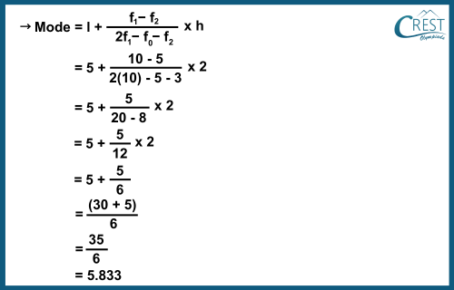
Explanation: Here the maximum class frequency is 10.

Thus, the modal class is 5 - 7.

We know that

Where

l (lower limit) = 5
h (class size) = 2
f₁ (frequency of the modal class) = 10
f₀ (frequency of the class preceding the modal class) = 5
f₂ (frequency of the class succeeding the modal class) = 3

Empirical Formula

There is an empirical relationship between the three measures of central tendency:

3 Median = Mode + 2 Mean

Example: What is the value of median if the values of mean and mode are 24 and 35 respectively?

a) 28.67
b) 27.67
c) 27.33
d) 28.33

Answer: b) 27.67

Explanation: We are given Mode = 35 and mean = 24

We know that 3 Median = Mode + 2 Mean

→ 3 Median = 35 + 2 (24)
              = 35 + 48
              = 83

→ Median = 83 / 3
           = 27.67

Quartiles

Quartiles divide a dataset into four equal parts or quarters. There are three quartiles - Q1, Q2 (also the median), and Q3 - representing specific points in a dataset when arranged in ascending order.

Lower Quartile (Q₁)

When the lower half, before the median, is divided into two equal parts, the value of the dividing variate is called the lower quartile. 

Let n terms be arranged in ascending order,

→ If n is even, then Q1 = (n / 4)th term.
→ If n is odd, then Q1 = [(n + 1) / 4]th term.

Upper Quartile (Q₃)

When the upper half, after the median, is divided into two equal parts, the value of the dividing variate is called the upper quartile. 

Let n terms be arranged in ascending order,

→ If n is even, then Q₃ = (3n / 4)^th term.
→ If n is odd, then Q₃ = [3(n + 1) / 4]^th term.

Inter-Quartile Range

It is the difference between the third quartile (Q₃) and the first quartile (Q₁).

Inter-Quartile Range = Q₃ − Q₁

→ Since Q₃ > Q₁, the inter-quartile range is always positive.

Example: What is the interquartile range for the data: 12, 5, 8, 17, 22, 15, 9, 11?

a) 9
b) 6
c) 7
d) 8

Answer: c) 7

Explanation: Inter-Quartile Range is the difference between the third quartile (Q₃) and the first quartile (Q₁).

Arrange the given data in ascending order.

5, 8, 9, 11, 12, 15, 17, 22

Thus, n = 8, which is an even number.

If n is even, then Q₁ = (n / 4)^th term.

→ Q₁ = (8 / 4)^th term
         = 2^nd term
         = 8

If n is even, then Q₃ = (3n / 4)^th term.

→ Q₃ = (3(8) / 4)^th term
         = 6^th term
         = 15

Inter-Quartile Range = Q₃ − Q₁
                               = 15 − 8
                               = 7

Graphical Representation

It refers to the visual depiction of data using graphs, charts, diagrams or other visual tools. Common types of graphical representations include bar graphs, histograms, line graphs and pie charts.

Histogram

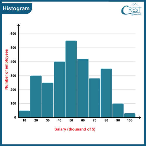
A histogram is a graphical representation of the distribution of numerical data, presented as a series of adjacent rectangles or bars. It displays the frequency of data within specified intervals along a continuous range.

In a histogram:

→ The horizontal axis represents the numerical range or intervals of the data.

→ The vertical axis shows the frequency of data points falling within each interval.

→ Bars are drawn adjacent to each other with widths representing the intervals and heights indicating the frequency of values within those intervals.

→ The bars have no gaps between them, as they represent continuous data ranges.

The histogram representing the salary distribution of employees of ABC Corporation is shown below:

Frequency Polygon

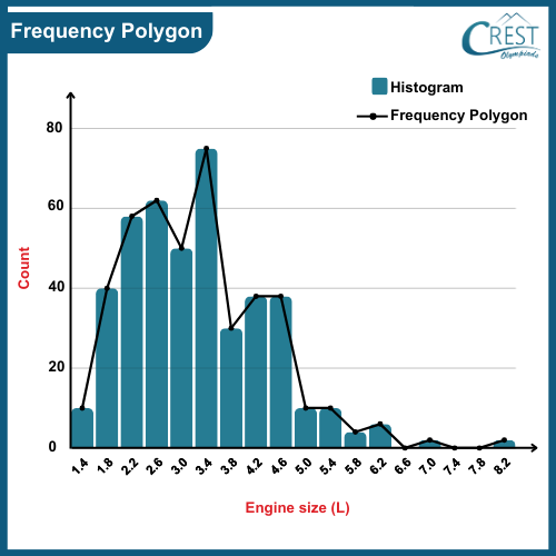
A frequency polygon is a graph that represents the frequency distribution of a dataset. It is created by connecting the midpoints of the tops of the bars in a histogram or the plotted points of a frequency table using straight-line segments.

In a frequency polygon:

→ The horizontal axis typically represents the variable being measured (such as values or intervals).

→ The vertical axis represents the frequency.

→ Points are plotted above the midpoint of each interval or value in the frequency distribution.

→ These points are connected by straight line segments to form a polygonal line, emphasising the pattern in the data's frequency distribution.

The frequency polygon representing the engine size of cars is shown below:

Ogive

An ogive, also known as a cumulative frequency curve, is a graphical representation that displays the cumulative frequencies of a dataset.

In an ogive:

→ The horizontal axis represents the variable being measured (values or intervals).

→ The vertical axis represents the cumulative frequency.

→ Points are plotted and connected to form a curve or line, indicating the cumulative total of frequencies up to that point.

→ The curve gradually rises, showing the increasing cumulative frequency as values progress.

The ogive of age of people attending library reading is shown below: